A common task in Computer Vision is to use a camera for localize and measure certain objects in the scene. In the industry is common to use images of objects on a high contrast background and use Computer Vision algorithms to extract useful information.
There’s a lot of literature about the computer vision algorithm that we can use to extract the information, but something that’s usually neglected is how to correctly setup the camera in order to correctly address the problem. This post aim is to shed light on this subject.
The problem
The problem we aim to solve with Computer vision is to measure (in mm) objects of unknown shape, but with known thickness \(T_o\) and max height \(H_o\) and width \(W_o\) values, while satisfying the constraint on the required minimum accuracy / error tolerance.
The camera setup for this kind of problem consists in:
- Finding the correct working distance (distance between the object surface and the lenses)
- Choose the right focal length.
In the following I’m going to show a possible 3 steps approach that can be used to correctly setup the camera.
Step 1: camera calibration & px/mm ratio calculation
Without entering in the detail of camera calibration, all we need to know is that the calibration process allow to represent the camera intrinsic parameters as a \(3 \times 3\) matrix. What the calibration does is to estimate the parameters of a pinhole camera model that approximate the camera that produces the set of photos given in input to the process.
\[A = \begin{pmatrix} f_x ~~\quad \gamma ~~\quad c_x \\ 0 ~~\quad f_y ~~\quad c_y \\ 0 ~~~\quad ~0 ~~\quad ~1 \end{pmatrix}\]where \(f_x\) and \(f_y\) are the focal distances in px and \((c_x, c_y)\) is the optical center in px.
In case of a squared sensor \(f_x\) and \(f_y\) are equal, but in general we can consider \(f_x \approx f_y\) and consider a single focal length in px
\[f_{xy} = \frac{f_x + f_y}{2} \quad [px]\]The theory of the camera resectioning gives us the relation between the estimated focal lengths (in px) and the real focal length (in mm).
\[f_x = m_x \cdot f \quad , \quad f_y = m_y \cdot f\]Since we’re considering \(f_{xy}\) we can just consider a single equation
\[f_{xy} = m \cdot f\]In short, the estimated focal length in pixel is the real focal length \(f\) (mm) times a scaling factor \(m\) (px/mm).
\[m = \frac{f_{xy}}{f} \quad [\frac{px}{mm}]\]This scaling factor is extremely important, because it measure the number of pixels in a millimeter of sensor.
Step 2: relationship between distance, object on sensor and object in scene
There’s a relation between the size of an object in the scene and the size of the object on the image plane. This relation comes from the thin lenses equiation.
Given \(X\) the real size of the object (mm) and \(x\) the size of the object in pixels, we know that
\[\text{WD} = \frac{X \cdot f}{\frac{x}{m}} \quad [\frac{mm^2}{\frac{px}{\frac{px}{mm}}} = mm]\]That in English it can be read as “the working distance in millimeters is the object real size in millimeter times the focal length in millimiters, divived by the object size on the image sensor”.
Hence it’s pretty easy to measure the size of the object in millimeters, when every other variable is know:
\[X = \frac{\text{WD} \cdot \frac{x}{m}}{f}\]Step 3: satisfy constraints
There are 2 constraints that have to be satisfied when designing an object measurement system:
- Being able to measure the whole object
- Minimum accuracy
Step 3.1: FOV constraint
The constraint on the ability of measure the whole object can be satisfied analyzing the Field of View (FOV) of the camera.
Let \(M_o = max(W_o, H_o) + \delta\), where \(\delta\) is a “safety margin” used to compensate the camera calibration distortion removal and the need for a background around the object (usual values for \(\delta\) are in range \([50, 100]\) mm). Let \(h\) and \(w\) be the height and width of the sensor respectively (these values are available on the camera datasheet), then
\[\alpha_H = FOV_H = 2\text{atan} \frac{h}{2f} \quad ,\quad \alpha_W = FOV_W = 2\text{atan} \frac{w}{2f}\]Since the object can be in any possible orientation we can consider only the smaller FOV when finding the right distance for the camera (because this is the constrained one):
\[\alpha = \min(\alpha_H, \alpha_W)\]It’s obvious that \(\alpha\) is the angle (in radians) between the working distance \(\text{WD}\) and the “last ray of light” (in the sense of farther from the center) captured by the sensor. It’s also clear that the length of this ray of light changes according to the working distance.
The following images will make everything clear:
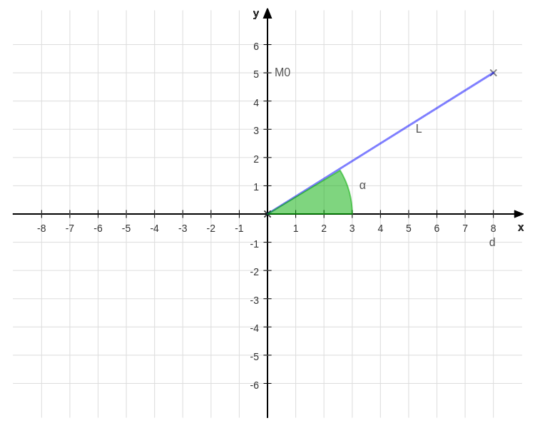
On the \(y\) axis the position of \(M_o\) is highlighted because we have to find the distance \(d\) that makes the whole object (and the safety margin) visible. Hence:
\[\begin{cases} WD \quad= L \cos \alpha \\ M_o \quad~~= L \sin \alpha \end{cases} \quad \Rightarrow \text{WD} = \frac{M_o}{\tan \alpha}\]This means that our working distance (noted as d in the picture) can be found exactly.
Please note that we’re creating an object measurement application, hence we can exploit other information regard the object in order to improve the precision. In fact, if we know in advance the set of thickness (in mm) \(T = \left\{T_1, T_2, \dots, T_n\right\}\) that our objects could have, we can place our camera at a smaller distance and hence increase the accuracy (see next section).
In practice, the real working distance (that’s the one we’re really interested) can be found as:
\[\text{WD}_r = \text{WD} - \min\{T\} \text{offset}\]The offset term is an optional term, that usually can be found on the camera datasheet, that’s the relative position of the sensor with respect to the measurement point (in the order of \([0, 5]\)mm usually).
WARNING: The working distance computed in this way is a theoretical estimation of the real working distance since the camera model we’re using is the pinhole using, hence we’re using the thin lens equation as the foundation for our reasoning. In practice, the working distance to use in a real-world application must be computed using a software solution (exploiting the information about the size of a known object and the measured object in pixel) since the thin lens equations can’t model complex lens system in a precise way. Hence, you can use all the content of this article to get a rough estimation of the working distance in order to properly setup the camera physically.
Step 3.2: minimum accuracy constraint
The constraint on the accuracy can be formalized as follow:
\[\frac{\#px}{\Delta} \geq 1\]where \(\Delta\) is the accuracy required and the 1 represents a lower bound (we can’t have a number of pixel less than 1 at a specified tolerance). In english: the number of pixel of the image per \(\Delta\) millimiter of the scene must be greather than 1.
If, for instance, the requirement is to have an accuracy of 3mm, the inequality becomes:
\[\frac{\#px}{3} \geq 1\]From the relation of the object in the scene on the object on the sensor (now with the real working distance) we can measure the number of pixels per millimiter, in fact
\[X = \frac{\text{WD}_r \cdot \frac{x}{m}}{f} \Leftrightarrow x = \frac{X f m}{\text{WD}_r} = \frac{Xf_{xy}}{\text{WD}_r}\]So, now is extremely easy to calculate the number of pixels per millimiter in the scene and check if the previous relation holds:
\[\frac{\Delta f m}{\text{WD}_r} \ge 1\]if the relation holds, we have correctly setup our system (but another safety margin can be to increase the number of pixels per accuracy required and hence change that 1 to something bigger).
Instead, if this relation does not hold we have to change the moving part of our system in order to satisfy every requirement:
- Check if the thickness of the object you’re measuring can help you making the camera closed to the object
- Change the focal length (and repeat every calculation, but only after a new calibration!)
- Evaluate the usage of more cameras and stitch the images together
- Last resort: change the camera(s)
One last tip: the relation \(x = \frac{X f m}{\text{WD}_r}\) allows also to measure the system accuracy (in px/mm), hence the number of pixels per single millimiter of the scene, just set \(\Delta=1\) and you’re done!
Disclosure
This article has been posted on the Zuru Tech Italy blog first and cross-posted here.