Autoencoders are neural networks models whose aim is to reproduce their input: this is trivial if the network has no constraints, but if the network is constrained the learning process becomes more interesting.
Simple Autoencoder
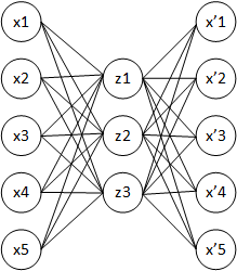
The simplest AutoEncoder (AE) has an MLP-like (Multi Layer Perceptron) structure:
- One input layer
- One hidden layer
- One output layer
The main difference between the AE and the MLP is that former’s output layer has the same cardinality of its input layer whilst the latter’s output layer cardinality is the number of classes the perceptron should be capable of classifying. Moreover, the AE belongs to the unsupervised learning algorithms family because it learns to represent unlabeled data; the MLP instead requires labeled data to be trained on.
The most important part of an AE is its hidden layer. In fact, this layer learns to encode the input whilst the output layer learns to decode it.
The hidden layer plays a fundamental role because a common application of AEs is dimensionality reduction: after the training phase, the output layer is usually thrown away and the AE is used to build a new dataset of samples with lower dimensions.
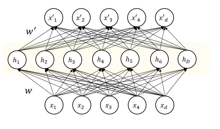
Formally:
- \(x \in [0,1]^{d}\) input vector
- \(W_i \in \mathbb{R}^{I_{di} \times O_{di}}\) parameters matrix of layer \(i\)-th, in charge of projecting a \(I_{di}\)-D input in a \(O_{di}\)-D space
- \(b_i \in \mathbb{R}^{O_{di}}\) bias vector
- \(a(h)\) activation function applied to every neuron of the layer \(h\).
The simplest AE can therefore be summarized as:
\[\begin{align} z &= a(xW_1 + b_1) \\ x' &= a(zW_2 + b_2) \end{align}\]The AE is the model that tries to minimize the reconstruction error between the input value \(x\) and the reconstructed value \(x'\): the training process is, therefore, the minimization of a \(L_p\) distance (like the \(L_2\)) or some other chosen metric.
\[\min \mathcal{L} = \min E(x, x') \stackrel{e.g.}{=} \min || x - x' ||_p\]From the information theory prospective the loss can be seen as:
\[\min \mathcal{L} = \min || x - \text{decode}(\text{encode}(x)) ||_p\]Constraints are everything
It can be easily noticed that if the number of units in the hidden layer is greater than or equal to the number of input units, the network will learn the identity function easily.
Learning the identity function alone is useless because the network will never learn to extract useful features but, instead, it will simply pass forward the input data to the output layer. In order to learn useful features, constraints must be added to the network: in this way no neuron can learn the identity function but they’ll learn to project inputs in a lower dimensional space.
AEs can extract the so-called latent variables from the input data. These variables are an aggregated view of the input data, that can be used to easily manage and understand the input data.
Dimensionality reduction using AEs leads to better results than classical dimensionality reduction techniques such as PCA due to the non-linearities and the type of constraints applied.
From the information theory point of view, the constraints force to learn a lossy representation of input data.
Number of hidden units
The simplest idea is to constrain the number of hidden units to be less than the number of input units.
\[|z| < d\]In this way, the identity function can’t be learned, but instead, a compress representation of the data should be.
Sparsity
To impose a sparsity constraint means to force some hidden unit to be inactive most of the time. The inactivity of a neuron \(i\) depends on the chosen activation function \(a_i(h)\).
If the activation function is the \(tanh\)
\[a_i(x) = \text{tanh}(x)\]being close to \(-1\) means to be inactive.
Sparsity is a desired characteristic for an autoencoder, because it allows to use a greater number of hidden units (even more than the input ones) and therefore gives the network the ability of learning different connections and extract different features (w.r.t. the features extracted with the only constraint on the number of hidden units). Moreover, sparsity can be used together with the constraint on the number of hidden units: an optimization process of the combination of these hyper-parameters is required to achieve better performance.
Sparsity can be forced adding a term to the loss function. Since we want that most of the neurons in the hidden layer are inactive, we can extract the average activation value for every neuron of the hidden layer (averaged over the whole training set \(TS\)) and force it to be under a threshold.
If the threshold value is low, the neurons will adapt their parameters (and thus their outputs) to respect this constraint. To do this, most of them will be inactive. Let:
\[\hat{\rho_{j}} = \frac{1}{|TS|} \sum_{i=1}^{|TS|}{a^{(2)}_j(x_i)}\]the average value for the \(j\)-th neuron of the hidden (number 2) layer.
Defining the sparsity parameter \(\rho\) as the desired average activation value for every hidden neuron and initializing it to a value close to zero, we can enforce the sparsity:
\[\hat{\rho}_{j} \le \rho \quad \forall j\]To achieve this, various penalization terms to the loss function can be added. The common one is based on the Kullback-Leibler (KL) divergence: a measure of the similarity of two distributions.
\[\sum_{j=1}^{O_{d_2}} \rho \log \frac{\rho}{\hat\rho_j} + (1-\rho) \log \frac{1-\rho}{1-\hat\rho_j} = \sum_{j=1}^{O_{d_2}} KL(\rho||\hat{\rho_j})\]In this case, the KL divergence is measured \(O_{d_2}\) times between a Bernoulli random variable with mean \(\rho\) and a Bernoulli random variable with mean \(\hat{\rho_j}\) used to model a single neuron.
In short, the \(KL\) divergence increase as the difference between \(\rho\) and \(\hat{\rho_j}\) increase. Therefore this is a good candidate to be added as penalization term to the loss, in that way the learning process via gradient descent will try to minimize the divergence while minimizing the reconstruction error.
The final form of the loss thus is:
\[\min \mathcal{L} = \min \left( E(x, x') + \sum_{j=1}^{O_{d_2}} KL(\rho||\hat{\rho_j}) \right)\]Adding noise: DAE
Instead of forcing the hidden layer to learn to extract features from the input data \(x\), we can train the AE to reconstruct the input from a corrupted version of it \(\tilde{x}\).
This allows the AE to discover more robust features w.r.t. the ones that could be learned from the original uncorrupted data.
This kind of constraint gave rise to the Denoising AutoEncoder (DAE) field.
DAEs have the same architecture of the AEs presented above, with just 2 differences:
- Input corruption step
- Loss function
Input corruption
For every element \(x\) in the training set, it’s required to generate a corrupted version.
\[\tilde{x} = \text{corrupt}(x)\]\(\text{corrupt}\) can be any function to corrupt the input data and it depends on the data type. For example, in the computer vision field can be added Gaussian noise or salt and pepper noise.
Moreover, AEs have been used to introduce the Dropout. Dropout is a simple technique to prevent neural networks from overfitting and it’s highly related to the input corruption: in fact, it consists of dropping out neurons (setting their output to \(0\)) casually with a specified probability.
Dropout is, therefore, an input corruption method and can be applied to improve the quality of the learned features of the hidden layer.
Loss function
Any loss function can be used, the only thing to pay attention to is the relations between the value to reconstruct.
In fact, we’re interested in minimizing the reconstruction error between the original input and the corrupted decoded output.
Therefore the minimization process should be:
\[\min \mathcal{L}(x, \tilde{x}') = \min || x - \text{decode}(\text{encode}(\text{corrupt}(x))) ||_p\]Common usage
As previously mentioned, autoencoders are commonly used to reduce the inputs’ dimensionality and not to decode the encoded value. The extracted compressed representation can be used for:
- Statistical analysis on the data distribution. At this purpose it possible to visualize a 2D representation using t-SNE
- Classification: classifiers works better with non-highly dimensional data
- One-Class Classification (OCC): if the AE has been trained on a single class only, it’s possible to find a threshold for the reconstruction error such that elements with a reconstruction error greater than this threshold expose differences from the learned model. It can somehow be seen as an outlier detection procedure.
Moreover, if the decoder has not been thrown away it can be used to perform Data denoising: if the AE trained is a DAE it has the ability to remove (some kind of) noise from the input, therefore a DAE can be used to do data preprocessing on a noisy source of data.
Next…
Autoencoders have been successfully applied to different tasks and different architecture have been defined.
In the next posts, I’ll introduce stacked autoencoders and convolutional autoencoders and I’ll mix them together to build a stacked convolutional autoencoder in Tensorflow.