The convolution operator allows filtering an input signal in order to extract some part of its content. Autoencoders in their traditional formulation do not take into account the fact that a signal can be seen as a sum of other signals. Convolutional Autoencoders, instead, use the convolution operator to exploit this observation. They learn to encode the input in a set of simple signals and then try to reconstruct the input from them.
Convolutions
A convolution in the general continue case is defined as the integral of the product of two functions (signals) after one is reversed and shifted:
\[f(t) * g(t) \stackrel{\text{def}}{=} \int_{-\infty}^{\infty}f(\tau)g(t-\tau)d\tau\]As a result, a convolution produces a new function (signal). The convolution is a commutative operation, therefore \(f(t) * g(t) = g(t) * f(t)\)
Autoencoders can be potentially trained to \(\text{decode}(\text{encode}(x))\) inputs living in a generic \(n\)-dimensional space. Practically, AEs are often used to extract features from 2D, finite and discrete input signals, such as digital images.
In the 2D discrete space, the convolution operation is defined as:
\[O(i, j) = \sum_{u=-\infty}^{\infty}\sum_{v=-\infty}^{\infty}F(u, v)I(i -u, j -v)\]In the image domain where the signals are finite, this formula becomes:
\[O(i, j) = \sum_{u=-2k-1}^{2k+1}\sum_{v=-2k -1}^{2k +1}F(u, v)I(i -u, j -v)\]Where:
- \(O(i,j)\) is the output pixel, in position \((i,j)\)
- \(2k +1\) is the side of a square, odd convolutional filter
- \(F\) is the convolutional filter
- \(I\) is the input image
This operation (single convolutional step) is done for every location \((i, j)\) of the input image \(I\) that completely overlaps with the convolutional filter as shown in Figure 1.
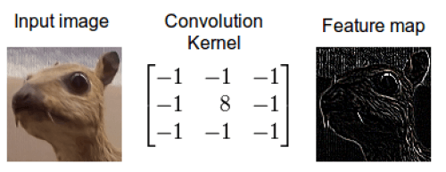
As it can be easily seen from the Figure 2 the result of a convolution depends on the value of the convolutional filter. There are different manually engineered convolutional filters, each one used in image processing tasks like denoising, blurring, etc…
The discrete 2D convolution has 2 additional parameters: Horizontal & Vertical Stride. They’re the number of pixels to skip along the dimensions of \(I\) after having performed a single convolutional step. Usually, the horizontal and vertical strides are equal and they’re noted as \(S\).
The result of a 2D discrete convolution of a square image with side \(I_w = I_h\) (for simplicity, but it’s easy to generalize to a generic rectangular image) with a squared convolutional filter with side \(2k + 1\) is a square image \(O\) with side:
\[O_w = O_h = \frac{I_w - (2k + 1)}{S} + 1 \quad \quad (1)\]Until now it has been shown the case of an image in gray scale (single channel) convolved with a single convolutional filter. If the input image has more than one channel, say \(D\) channels, the convolution operator spans along any of these channels.
The general rule is that a convolutional filter must have the same number of channels of the image is convolved with. It’s possible to generalize the concept of discrete 2-D convolution, treating stacks of 2D signals as volumes.
Convolution among volumes
A volume is a rectangular parallelepiped completely defined by the triple \((W, H, D)\), where:
- \(W \ge 1\) is its width
- \(H \ge 1\) is its height
- \(D \ge 1\) is its depth
It’s obvious that a gray-scale image can be seen as a volume width \(D=1\) whilst an RGB image can be seen as a volume with \(D=3\).
A convolutional filter can be also seen as a volume of filters with depth \(D\). In particular, we can think about the image and the filter as a set (the order doesn’t matter) of single-channel images/filters.
\[I = \left\{I_1,\cdots, I_D\right\}, \quad F = \left\{F_1, \cdots, F_D\right\}\]It’s possible to generalize the previous convolution formula, in order to keep in account the depths:
\[O(i, j) = \sum_{d=1}^{D}{\sum_{u=-2k-1}^{2k+1}\sum_{v=-2k -1}^{2k +1}F_d(u, v)I_d(i -u, j -v)}\]The result of a convolution among volumes is called activation map. The activation map is a volume with \(D=1\).
It may sound strange that a 2D convolution is done among volumes that are 3D objects. In reality, for an input volume with depth \(D\) exactly \(D\) 2D discrete convolutions are performed. The sum (collapse) of the \(D\) activation maps produced is a way to treat this set of 2D convolutions as a single 2D convolution. In this way, every single position \((i,j)\) of the resulting activation map \(O\) contains the information extracted from the same input location through its whole depth.
Intuitively, one can think about this operation as a way to keep into account the relations that exist along the RGB channels of a single input pixel.
Convolutional AutoEncoders
Convolutional AutoEncoders (CAEs) approach the filter definition task from a different perspective: instead of manually engineer convolutional filters we let the model learn the optimal filters that minimize the reconstruction error. These filters can then be used in any other computer vision task.
CAEs are the state-of-art tools for unsupervised learning of convolutional filters. Once these filters have been learned, they can be applied to any input in order to extract features. These features, then, can be used to do any task that requires a compact representation of the input, like classification.
CAEs are a type of Convolutional Neural Networks (CNNs): the main difference between the common interpretation of CNN and CAE is that the former are trained end-to-end to learn filters and combine features with the aim of classifying their input. In fact, CNNs are usually referred as supervised learning algorithms. The latter, instead, are trained only to learn filters able to extract features that can be used to reconstruct the input.
CAEs, due to their convolutional nature, scale well to realistic-sized high-dimensional images because the number of parameters required to produce an activation map is always the same, no matter what the size of the input is. Therefore, CAEs are general purpose feature extractors differently from AEs that completely ignore the 2D image structure. In fact, in AEs the image must be unrolled into a single vector and the network must be built following the constraint on the number of inputs. In other words, AEs introduce redundancy in the parameters, forcing each feature to be global (i.e., to span the entire visual field)1, while CAEs do not.
Encode
It’s easy to understand that a single convolutional filter, can’t learn to extract the great variety of patterns that compose an image. For this reason, every convolutional layer is composed of \(n\) (hyper-parameter) convolutional filters, each with depth \(D\), where \(D\) is the input depth.
Therefore, a convolution among an input volume \(I = \left\{I_1,\cdots, I_D\right\}\) and a set of \(n\) convolutional filters \(\left\{F^{(1)}_1, \cdots, F^{(1)}_n\right\}\), each with depth \(D\), produces a set of \(n\) activation maps, or equivalently, a volume of activations maps whith depth \(n\):
\[O_m(i, j) = a\left(\sum_{d=1}^{D}{\sum_{u=-2k-1}^{2k+1}\sum_{v=-2k -1}^{2k +1}F^{(1)}_{m_d}(u, v)I_d(i -u, j -v)}\right) \quad m = 1, \cdots, n\]To improve the generalization capabilities of the network, every convolution is wrapped by a non-linear function \(a\) (activation), in that way the training procedure can learn to represent input combining non-linear functions:
\[z_m = O_m = a(I * F^{(1)}_{m} + b^{(1)}_m) \quad m = 1, \cdots, m\]Where \(b^{(1)}_m\) is the bias (single real value for every activation map) for the \(m\)-th feature map. The term \(z_m\) has been introduced to use the same variable name for the latent variable used in the AEs.
The produced activation maps are the encoding of the input \(I\) in a low dimensional space; a dimension that’s not the dimension (width and height) of \(O\) but the number of parameters used to build every feature map \(O_m\), in other words, the number of parameters to learn.
Since our objective is to reconstruct the input \(I\) from the produced feature maps, we want a decoding operation capable of doing this. Convolutional autoencoders are fully convolutional networks, therefore the decoding operation is again a convolution.
A careful reader could argue that the convolution reduces the output’s spatial extent and therefore is not possible to use a convolution to reconstruct a volume with the same spatial extent of its input.
This is true, but we can work around this issue using the input padding. If we pad with zeros the input volume \(I\), then the result of the first convolution can have a spatial extent greater than the one of \(I\) and thus the second convolution can produce a volume with the original spatial extent of \(I\).
Therefore, the amount of zeros we want to pad the input with is such that:
\[\text{dim}(I) = \text{dim}(\text{decode}(\text{encode}(I)))\]It follows from the equation 1 that we want to pad \(I\) by \(2(2k + 1) - 2\) zeros (\((2k + 1) - 1\) per side), in that way the encoding convolution will produce a volume with width and height equals to
\[O_w = O_h = (I_w + 2(2k +1) -2) - (2k + 1) + 1 = I_w + (2k + 1) - 1\]Decode
The produced \(n\) feature maps \(z_{m=1,\cdots,n}\) (latent representations) will be used as input to the decoder, in order to reconstruct the input image \(I\) from this reduced representation.
The hyper-parameters of the decoding convolution are fixed by the encoding architecture, in fact:
- Filters volume \(F^{(2)}\) with dimensions \((2k +1 , 2k+1 , n)\), because the convolution should span across every feature map and produce a volume with the same spatial extent of \(I\)
- Number of filters to learn: \(D\), because we’are interested in reconstructing the input image that has depth \(D\)
Therefore, the reconstructed image \(\tilde{I}\) is the result of the convolution between the volume of feature maps \(Z = \{z_{i=1}\}^{n}\) and this convolutional filters volume \(F^{(2)}\).
\[\tilde{I} = a(Z * F^{(2)}_{m} + b^{(2)})\]Padding \(I\) with the previously found amount of zeros, leads the decoding convolution to produce a volume with dimensions:
\[O_w = O_h = ( I_w + (2k + 1) - 1 ) - (2k + 1) + 1 = I_w = I_h\]Having input’s dimensions equals to the output’s dimensions, it possible to relate input and output using any loss function, like the MSE:
\[\mathcal{L}(I, \tilde{I}) = \frac{1}{2} || I - \tilde{I}||_{2}^{2}\]Next…
In the following post, I’ll show how to build, train and use a convolutional autoencoder with Tensorflow. The following posts will guide the reader deep down the deep learning architectures for CAEs: stacked convolutional autoencoders.