After being interrupted dozens of times a day while coding with my headphones on, I decided to find a solution that eliminates the stress of pausing and re-playing the song I was listening to.
The idea is trivial:
- When you’re in front of your PC with your headphones on: the music plays.
- Someone interrupts you, and you have to remove your headphones: the music pauses.
- You walk away from your PC: the music pauses.
- You come back to your PC, and you put the headphones on: the music plays again.
- If you want to manually control the player, the manual control has the precedence; e.g. if you have your headphones off and you press play, the music plays as you expect.
The idea is trivial, yes, but implementing it has been fun and challenging at the same time.
In this article I’m going to describe the software architecture and the implementation details of this application named FaceCTRL.
Note: if you’re not interested in all the implementation details, you can simply go on Github (galeone/facectrl) or even just pip install facectrl and use it.
Overview
Let’s start by looking at the final result: below you can see how FaceCTRL works when launched in debug mode.
In the following we will analyze the steps required to build this application.
Problem definition and analysis
The goal of this application is pretty clear: we have to detect if the person in front of the cameras wears headphones and control the chosen media player depending on the presence/absence of the person and of his/her headphones.
The goal, thus, can be divided in two different parts. The computer vision part dedicated to image processing and understanding, and the media player part dedicated to the control of the media player given the output of the computer vision analysis.
Focusing on the first part of the problem, we can define a computer vision pipeline that works on a video stream. In particular, we expect the pipeline to do:
- Face detection: detect and localize a face in the video stream: we must be sure that someone is in front of the camera.
- Face tracking: the face detection task is usually implemented using neural networks or other traditional methods that, often, are not adequate for a real-time application. Thus, we have to use a tracking algorithm to track the detected face.
- Classification: while tracking we have to understand if the person is wearing headphones.
The problem of detecting a face in an image is a traditional computer vision problem and as such, there exist several face detection algorithms ready to use that work pretty well. The same reasoning applies to the face tracking, there are several trackers ready to use that are fast, accurate, and robust to subject transformations and occlusions.
The problem of detecting when a person wears headphones, instead, can be modeled in two different ways:
-
One class classification / Anomaly detection. If we follow this path, we must train a model on positive samples only (headphones on), and then use the trained model to detect anomalies.
- Pros: we can detect when the person is wearing headphones.
- Cons: we only know the result is anomalous when we detect an anomaly; we don’t know if this is because the person has no headphones, or because there is no one in front of the camera.
-
Binary classification. We must assume that the only possible outcomes of this problem are two: headphones on and headphones off.
- Pros: we can detect when the person is wearing and not warning headphones.
- Cons: we can’t detect anomalous situation: the outcome will always be headphones on/off even if there’s no one in front of the camera.
In the following we will see how to implement and end-to-end solution to solve this classification problem, from the dataset creation to the model definition, training and inference.
We now have an idea of the problem we want to solve: we know from an high level perspective what’s the architecture we expect for the computer vision / machine learning pipeline.
How should we define, instead, the media player control part? The second part of the problem, thus, is the development of an application that:
- Knows how to communicate with a media player: is the media player running?
- Knows how to play/pause/stop the music.
- It allows us to receive change of status (e.g. the person while still wearing headphones pressed the pause button - we don’t want to automatically restart the music only because he/she still has headphones on)
Moreover, the computer vision pipeline and media player control must work concurrently and communicate any status change almost in real time.
From the problem definition, is pretty clear that we want to develop a real time application. This requirement imposes constraints on both the computer vision and media player control parts.
Software architecture
The software architecture naturally follows from the analysis of the requirements presented above. The diagram below shows the high level architecture, without any implementation detail.
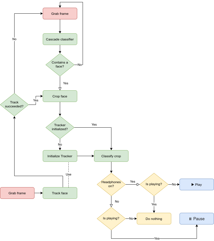
The red blocks are the inputs. In practice, these are implemented as a separate thread that always grab frames freely, without waiting for the image processing pipeline.
The green blocks represent the computer vision and machine learning inference pipeline.
The yellow blocks represent the media player control pipeline.
To conclude, the blue blocks are the actions: in practice FaceCTRL only has two output actions: play and pause.
Without digging too much into the implementation details (you can have a look at the complete source code on Github), we just want to emphasize that the whole green part is the machine learning inference pipeline, and below present some of the building blocks of the architecture.
Computer Vision pipeline
We want to have a lightweight image processing pipeline, thus we need the face detection and tracking blocks that:
- Execute in real time, thus a fast execution.
- Have a low memory footprint.
At this purpose, OpenCV offers us a whole set of ready to use Haar Feature-based cascade classifiers trained to detect faces. These classifiers work on a pyramid of images and thus, the classifiers themselves are capable of working efficiently on images with different resolutions. OpenCV (note: not the python module, you need OpenCV installed system-wise) comes with this pre-trained models ready to use, we only need to load the parameters from XML files.
We can thus define a FaceDetector class that abstracts the features we need. The most important part of the code below (file detector.py), is the usage of cv2.CascadeClassifier.detectMultiScale method, that executes the cascade classification on the image pyramid.
The crop method, instead, has the expansion parameter that’s useful since we’re interested in detecting not only the face, but also the headphones. For this reason we want to expand the detected bounding box by a certain amount.
from pathlib import Path
from typing import Tuple

import cv2
import numpy as np


class FaceDetector:
    """Initialize a classifier and uses it to detect the bigger
    face present into an image.
    """

    def __init__(self, params: Path) -> None:
        """Initializes the face detector using the specified parameters.

        Args:
            params: the path of the haar cascade classifier XML file.
        """
        self.classifier = cv2.CascadeClassifier(str(params))

    def detect(self, frame: np.array) -> Tuple:
        """Search for faces into the input frame.
        Returns the bounding box containing the bigger (close to the camera)
        detected face, if any.
        When no face is detected, the tuple returned has width and height void.

        Args:
            frame: the BGR input image.
        Returns:
            (x,y,w,h): the bounding box.
        """

        frame = cv2.cvtColor(frame, cv2.COLOR_BGR2GRAY)
        proposals = np.array(
            self.classifier.detectMultiScale(
                frame,
                scaleFactor=1.5,  # 50%
                # that's big, but we're interested
                # in detecting faces closes to the camera, so
                # this is OK.
                minNeighbors=4,
                # We want at least "minNeighbors" detections
                # around the same face,
                minSize=(frame.shape[0] // 4, frame.shape[1] // 4),
                # Only bigger faces -> we suppose the face to be at least
                # 25% of the content of the input image
                maxSize=(frame.shape[0], frame.shape[1]),
            )
        )

        # If faces have been detected, find the bigger one
        if proposals.size:
            bigger_id = 0
            bigger_area = 0
            for idx, (_, _, width, height) in enumerate(proposals):
                area = width * height
                if area > bigger_area:
                    bigger_id = idx
                    bigger_area = area
            return tuple(proposals[bigger_id])  # (x,y,w,h)
        return (0, 0, 0, 0)

    @staticmethod
    def crop(frame, bounding_box, expansion=(0, 0)) -> np.array:
        """
        Extract from the input frame the content of the bounding_box.
        Applies the required expension to the bounding box.

        Args:
            frame: BGR image
            bounding_box: tuple with format (x,y,w,h)
            expansion: the amount of pixesl the add to increase the
                       bouding box size, from the center.
        Returns:
            cropped: BGR image with size, at least (bounding_box[2], bounding_box[3]).
        """

        x, y, width, height = [
            int(element) for element in bounding_box
        ]  # pylint: disable=invalid-name

        if x < 0:
            x = 0
        if y < 0:
            y = 0

        halfs = (expansion[0] // 2, expansion[1] // 2)
        if width + halfs[0] <= frame.shape[1]:
            width += halfs[0]
        if x - halfs[0] >= 0:
            x -= halfs[0]
        if height + halfs[1] <= frame.shape[0]:
            height += halfs[1]
        if y - halfs[1] >= 0:
            y -= halfs[1]

        image_crop = frame[y : y + height, x : x + width]
        return image_crop
Also for the face tracking, OpenCV (note: in its contrib module) offers a long list of object tracking algorithms already implemented and ready to use. A nice analysis of the trackers has been made by Adrian Rosebrock here. We decided to use the CSRT tracking algorithm because it’s fast enough and it successfully tracks the face even when rotated.
From the flowchart, it’s also clear that the tracker must use a trained classifier (to classify if the subject wears the headphones) and use it to classify the tracked object. In the snippet below (file tracker.py) you can also see how we handle the tracking failures (the person covers the webcam or walks away) using a threshold; the most important method here is track_and_classify.
It’s also pretty clear that we abstracted the classifier results using the Enum class ClassificationResult (not reported in this article for brevity).
from typing import Tuple

import cv2
import numpy as np

from facectrl.ml import ClassificationResult, Classifier, FaceDetector

class Tracker:
    """Tracks one object. It uses the CSRT tracker."""

    def __init__(
        self, frame, bounding_box, max_failures=10, debug: bool = False,
    ) -> None:
        """Initialize the frame tracker: start tracking the object
        localized into the bounding box in the current frame.
        Args:
            frame: BGR input image
            bounding_box: the bounding box containing the object to track
            max_failures: the number of frame to skip, before raising an
                          exception during the "track" call.
            debug: set to true to enable visual debugging (opencv window)
        Returns:
            None
        """
        self._tracker = cv2.TrackerCSRT_create()
        self._golden_crop = FaceDetector.crop(frame, tuple(bounding_box))
        self._tracker.init(frame, bounding_box)
        self._max_failures = max_failures
        self._failures = 0
        self._debug = debug
        self._classifier = None

    def track(self, frame) -> Tuple[bool, Tuple]:
        """Track the object (selected during the init), in the current frame.
        If the number of attempts of tracking exceed the value of max_failures
        (selected during the init), this function throws a ValueError exception.
        Args:
            frame: BGR input image
        Returns:
            success, bounding_box: a boolean that indicates if the tracking succded
            and a bounding_box containing the tracked objecrt positon.
        """
        return self._tracker.update(frame)

    @property
    def classifier(self) -> Classifier:
        """Get the classifier previousluy set. None otherwise."""
        return self._classifier

    @classifier.setter
    def classifier(self, classifier: Classifier) -> None:
        """
        Args:
            classifier: the Classifier to use
        """
        self._classifier = classifier

    @property
    def max_failures(self) -> int:
        """Get the max_failures value: the number of frame to skip
        before raising an exception during the "track" call."""
        return self._max_failures

    @max_failures.setter
    def max_failures(self, value):
        """Update the max_failures value."""
        self._max_failures = value

    def track_and_classify(
        self, frame: np.array, expansion=(100, 100)
    ) -> ClassificationResult:
        """Track the object (selected during the init), in the current frame.
        If the number of attempts of tracking exceed the value of max_failures
        (selected during the init), this function throws a ValueError exception.
        Args:
            frame: BGR input image
            expansion: expand the ROI around the detected object by this amount
        Return:
            classification_result (ClassificationResult)
        """
        if not self._classifier:
            raise ValueError("You need to set a classifier first.")
        success, bounding_box = self.track(frame)
        classification_result = ClassificationResult.UNKNOWN
        if success:
            self._failures = 0

            crop = FaceDetector.crop(frame, bounding_box, expansion=expansion)
            classification_result = self._classifier(self._classifier.preprocess(crop))[
                0
            ]
        else:
            self._failures += 1
            if self._failures >= self._max_failures:
                raise ValueError(f"Can't find object for {self._max_failures} times")

        return classification_result
The third and last part of the image processing pipeline is the classification of the tracked subject. Since we want our model for the classification to be fast (since we want to use it on every frame, while tracking) we have to design a model that:
- Contains few operations.
- Is lightweight.
- Can be exported in an optimized format designed to speed up the inference.
Thus, we can try to reduce the number of parameters of the model and reduce the memory footprint assuming that every image is in gray scale, in the end, the presence or the absence of the headphones doesn’t depend on the color information.
Moreover, since we want to work only with the information contained into the bounding box, we can set a small and fixed input shape for our model. Thus we decide for an input resolution of \(64 \times 64 \times 1\) for the classification model. All the pre-processing steps are executed by the static method Classifier.preprocess(crop).
In the section Machine learning pipeline we will see the various steps required to get the data, create the dataset, train the model and export it for inference.
Media player control
The media player control module comes almost for free thanks to the amazing project Playerctl. From the doc:
Playerctl is a command-line utility and library for controlling media players that implement the MPRIS D-Bus Interface Specification. Playerctl makes it easy to bind player actions, such as play and pause, to media keys.
The amazing part is the availability of the Python bindings, that allows using this GLib application in a straightforward way.
In fact, this GLib application allows us to trigger events and to take actions when an event occurs (the application exposes certain “signals” and we can “connect” functions to thems).
Without describing the whole player control module (file ctrl.py), we can focus on the main method that controls the media player using the computer vision. The player control waits for the event name-appeared (a new media player signaled its presence), and if the player name matches the one specified by the user, then it calls the _start() method. This method uses the VideoStream context manager (self._stream variable; file stream.py), this object is the implementation of the “red box” in the flowchart; thus it creates a separate thread that is never slowed-down by the image processing pipeline. Moreover, it only acquires the resource (the webcam) when the player starts.
def _start(self) -> None:
    with self._stream:
        while not self._is_stopped() and self._player:
            classification_result = ClassificationResult.UNKNOWN
            # find the face for the first time in this loop
            logging.info("Detecting a face...")
            start = time()
            while (
                classification_result == ClassificationResult.UNKNOWN
                and self._player
            ):
                frame = self._stream.read()

                # More than 2 seconds without a detected face: pause
                if (
                    self._is_playing()
                    and time() - start > 2
                    and not self._is_stopped()
                ):
                    logging.info("Nobody in front of the camera")
                    self._pause_player()
                    sleep(1)

                classification_result, bounding_box = self._detect_and_classify(
                    frame
                )

            previous_result = classification_result
            self._decide(classification_result, previous_result)

            tracker = Tracker(
                frame,
                bounding_box,
                # Halve the FPS value because at this time, self.fps
                # Is the VideoStream FPS - without taking into account the
                # image processing.
                max_failures=self._fps_value() // 2,
                debug=self._debug,
            )
            tracker.classifier = self._classifier

            try:
                # Start tracking stream
                frame_counter = 0
                while not self._is_stopped() and self._player:
                    if self._fps < 0:
                        start = time()
                    frame = self._stream.read()
                    classification_result = tracker.track_and_classify(
                        frame, expansion=self._expansion
                    )
                    self._decide(classification_result, previous_result)
                    previous_result = classification_result
                    if self._fps < 0:
                        frame_counter += 1
                        if time() - start >= 1:
                            self._fps = frame_counter
                            # Update tracker max_failures
                            tracker.max_failures = self._fps_value()

            except ValueError:
                logging.info("Tracking failed")
                self._pause_player()
When it’s time to take an action, the decide method is invoked. This method contains all the logic of control of the media-player. In order to deal with the possible false positives, we implemented a simple “voting” system. We take an action if and only if the predictions made during the last second (thus, on all the frame viewed in that second) are all equals.
def _decide(
    self,
    classification_result: ClassificationResult,
    previous_result: ClassificationResult,
) -> None:
    if classification_result == previous_result:
        self._counters[classification_result] += 1
    else:
        for hit in ClassificationResult:
            self._counters[hit] = 0

    # Stabilize the predictions: take a NEW action only if all the latest
    # predictions agree with this one
    if self._counters[classification_result] >= self._fps_value():
        if self._is_playing():
            logging.info("is playing")
            if classification_result in (
                ClassificationResult.HEADPHONES_OFF,
                ClassificationResult.UNKNOWN,
            ):
                logging.info("decide: pause")
                self._pause_player()
                return
        elif self._is_stopped() or self._is_paused():
            logging.info("is stopped or paused")
            if classification_result == ClassificationResult.HEADPHONES_ON:
                logging.info("decide: play")
                self._play_player()
                return

    logging.info("decide: dp nothing")
As it can be easily seen, controlling the media player is easy; but of course the quality of the control depends on the quality of the classifier.
Machine learning pipeline
The most important part of every machine learning project is the data. Thus, since from the software architecture we know that our classifier should be able to classify the face while being tracked, a good idea is to create a dataset using the tracker itself (file dataset.py):
import os
import sys
import time
from argparse import ArgumentParser
from pathlib import Path

import cv2
import numpy as np

from facectrl.ml import FaceDetector
from facectrl.video import Tracker, VideoStream


class Builder:
    """Builds the dataset interactively."""

    def __init__(self, dest: Path, params: Path, src: int = 0) -> None:
        """Initializes the dataset builder.

        Args:
            dest: the destination folder for the dataset.
            params: Path of the haar cascade classifier parameters.
            src: the ID of the video stream to use (input of VideoStream).
        Returns:
            None
        """
        self._on_dir = dest / "on"
        self._off_dir = dest / "off"
        if not self._on_dir.exists():
            os.makedirs(self._on_dir)
        if not self._off_dir.exists():
            os.makedirs(self._off_dir)
        self._stream = VideoStream(src)
        self._detector = FaceDetector(params)

    def _acquire(self, path, expansion, prefix) -> None:
        """Acquire and store into path the samples.
        Args:
            path: the path where to store the cropped images.
            expansion: the expansion to apply to the bounding box detected.
            prefix: prefix added to the opencv window
        Returns:
            None
        """
        i = 0
        quit_key = ord("q")
        start = len(list(path.glob("*.png")))
        with self._stream:
            detected = False
            while not detected:
                frame = self._stream.read()
                bounding_box = self._detector.detect(frame)
                detected = bounding_box[-1] != 0

            tracker = Tracker(frame, bounding_box)
            success = True
            while success:
                success, bounding_box = tracker.track(frame)
                if success:
                    bounding_box = np.int32(bounding_box)
                    crop = FaceDetector.crop(frame, bounding_box, expansion)
                    crop_copy = crop.copy()
                    cv2.putText(
                        crop_copy,
                        f"{prefix} {i + 1}",
                        (30, crop.shape[0] - 30),
                        cv2.FONT_HERSHEY_SIMPLEX,
                        fontScale=1,
                        color=(0, 0, 255),
                        thickness=2,
                    )
                    cv2.imshow("grab", crop_copy)
                    key = cv2.waitKey(1) & 0xFF
                    if key == quit_key:
                        success = False
                    cv2.imwrite(str(path / Path(str(start + i) + ".png")), crop)
                    i += 1
                frame = self._stream.read()
        cv2.destroyAllWindows()

    def headphones_on(self, expansion=(70, 70)) -> None:
        """Acquire and store the images with the headphones on.
        Args:
            expansion: the expansion to apply to the bounding box detected.
        Returns:
            None
        """
        return self._acquire(self._on_dir, expansion, "ON")

    def headphones_off(self, expansion=(70, 70)) -> None:
        """Acquire and store the images with the headphones off.
        Args:
            expansion: the expansion to apply to the bounding box detected.
        Returns:
            None
        """
        return self._acquire(self._off_dir, expansion, "OFF")
Using this class is it possible to create a dataset that contains images with different appearences, with frontal face, lateral face, blurred by the motion, and so on.
The DatasetBuilder class, instead, can be used to create a tf.data.Dataset, that is an highly optimized and flexible object to create data input pipeline (file train.py):
class DatasetBuilder:
    @staticmethod
    def _to_image(filename: str) -> tf.Tensor:
        """Read the image from the path, and returns the resizes (64x64) image."""

        image = tf.io.read_file(filename)
        image = tf.image.decode_png(image)
        image = tf.image.rgb_to_grayscale(image)
        image = tf.image.convert_image_dtype(image, tf.float32)
        image = tf.image.resize(image, (64, 64))
        return image

    @staticmethod
    def augment(image: tf.Tensor) -> tf.Tensor:
        """Given an image, returns a batch with all the tf.image.random*
        transformation applied.
        Args:
            image (tf.Tensor): the input image, 3D tensor.

        Returns:
            images (tf.Tensor): 4D tensor.
        """
        return tf.stack(
            [
                tf.image.random_flip_left_right(image),
                tf.image.random_contrast(image, lower=0.1, upper=0.6),
                tf.image.random_brightness(image, max_delta=0.2),
                tf.image.random_jpeg_quality(
                    image, min_jpeg_quality=20, max_jpeg_quality=100
                ),
            ]
        )

    def __call__(
        self,
        glob_path: Path,
        batch_size: int,
        augmentation: bool = False,
        use_label: int = -1,
        skip: int = -1,
        take: int = -1,
    ) -> tf.data.Dataset:
        """Read all the images in the glob_path, and optionally applies
        the data agumentation step.
        Args:
            glob_path (Path): the path of the captured images, with a glob pattern.
            batch_size (int): the batch size.
            augmentation(bool): when True, applies data agumentation and increase the
                                dataset size.
            skip: how many files to skip from the glob_path listed files. -1 = do not skip.
            take: how many files to take from the glob_path listed files. -1 = take all.
        Returns:
            the tf.data.Dataset
        """
        dataset = tf.data.Dataset.list_files(str(glob_path)).map(self._to_image)

        if skip != -1:
            dataset = dataset.skip(skip)
        if take != -1:
            dataset = dataset.take(take)

        if augmentation:
            dataset = dataset.map(self.augment).unbatch()
            # 4 because augment increase the dataset size by 4
            dataset = dataset.shuffle(4 * len(glob(str(glob_path))))
        if use_label != -1:
            label = use_label
            dataset = dataset.map(lambda image: (image, label))
        else:
            dataset = dataset.map(self._to_autoencoder_format)
        return dataset.batch(batch_size).prefetch(1)
We now have the dataset and a class able to create the input pipelines (the take and skip method of tf.data.Dataset can be easily used to create train/validation/test splits), we only need to create a small model.
In this article we present only the classification model, but in the repository you can find:
- The classifier (binary classification problem)
- The autoencoder (anomaly detection)
- The variational autoencoder (anomaly detection)
All the models have been implemented using the Keras model subclassing API, and converted in the optimized format for inference (the SavedModel file format) thanks to the @tf.function decorator. In fact, when we decorate a method using @tf.function we are implicitly telling to TensorFlow to convert it to its graph representation and to use, during the export phase, the built graphs to create the SavedModel.
Because of the requirements on the model, we defined it in the most simple possible way: just two Dense layers. The output layer is linear since we delegate to the loss function the application of the correct non linearity during the training phase (file model.py).
class NN(tf.keras.Model):
    def __init__(self):
        super().__init__()
        self._model = tf.keras.Sequential(
            [
                tf.keras.layers.Input(shape=(64, 64, 1)),
                tf.keras.layers.Flatten(),
                tf.keras.layers.Dense(64, activation=tf.nn.leaky_relu),
                tf.keras.layers.Dense(2),
            ]
        )

    @tf.function
    def call(self, inputs, training):
        return self._model(inputs, training)
Our goal for the training phase is to select the model that better classifies the validation data. Thus, we have first to create the train/validation datasets and then measure the binary accuracy at the end of every epoch and select, thus, the model with the highest validation accuracy (model selection phase).
In order to do this in the most simplified way, we decided to use AshPy (disclaimer: I’m one of the authors). From the doc:
AshPy is a TensorFlow 2.1 library for (distributed) training, evaluation, model selection, and fast prototyping. It is designed to ease the burden of setting up all the nuances of the architectures built to train complex custom deep learning models.
After creating the training_dataaset and the validation_dataset using the DatasetBuilder, it is possible to train the model and do model selection in a few lines with this library(file train.py):
model = NN()
loss = ClassifierLoss(
    tf.keras.losses.SparseCategoricalCrossentropy(from_logits=True)
)
metrics = [
    ClassifierMetric(
        tf.keras.metrics.BinaryAccuracy(), model_selection_operator=operator.gt
    )
]
best_path = logdir / "on" / "best" / "binary_accuracy"
best_json = "binary_accuracy.json"
The ClassifierLoss and ClassifierMetric objects are provided by AshPy. Interestingly, the ClassifierMetric offers the model_selection_operator parameter, that allows us to specify the operator for doing (and enabling) model selection on that metric. The "best" model, is saved in the best_path folder, together with a JSON file that contains the metric information (step, value reached, …).
Training the model is just a matter of instantiating and calling the correct “trainer”, in this case the ClassifierTrainer.
# define the model by passing a dummy input to
# the call method of the Model
model(tf.zeros((1, 64, 64, 1)), training=True)
model.summary()

learning_rate = tf.keras.optimizers.schedules.ExponentialDecay(
    5e-3, decay_rate=0.98, decay_steps=1000, staircase=True
)
trainer = ClassifierTrainer(
    model=model,
    metrics=metrics,
    optimizer=tf.optimizers.Adam(learning_rate),
    loss=loss,
    logdir=str(logdir / "on"),
    epochs=epochs,
)

trainer(training_dataset, validation_dataset, measure_performance_freq=-1)
AshPy did all the work for us and we have in our best_folder the model that reached the best validation accuracy, that 1.0 in this case (but remember, this is a very small dataset and the validation dataset too has a low variance and perhaps is not representative of the population).
Now, since it is required to export the model in a format optimized for the inference, the choice naturally goes to the SavedModel serialization format. This file format is designed to be portable and lightweight, and the TensorFlow ecosystem offers us a whole set of platform able to use it. The very same SavedModel can be used in Python, C++, Go, TensorFlow serving, and many other platforms.
We can now restore this model and convert it in a SavedModel by passing it to the tf.saved_model.save function. To correctly restore the model we use the ClassifierRestore offered by AshPy.
# Restore the best model and save it as a SavedModel
model = ClassifierRestorer(str(best_path)).restore_model(model)
# Define the input shape by calling it on fake data
model(tf.zeros((1, 64, 64, 1)), training=False)
model.summary()

dest_path = logdir / "on" / "saved"
tf.saved_model.save(model, str(dest_path))
This saved model can now be loaded and plugged in into the Classifier class (not presented here), the simply invokes the serialized call method to get the predictions.
Putting the pieces together and adding a simple CLI interface, we now have FaceCTRL ready to use.
Conclusion
In this article we described some of the steps followed to develop FaceCTRL. The application is in its alpha version and it requires improvements, new features (what about changing song with the hands?) and a lot of new data.
Thus, if you find this project interesting and you want to contribute somehow (improving the code, submit your dataset, …), please open an issue on Github and let’s work together.