DISCLAIMER: The code used in this article refers to an old version of DTB (now also renamed DyTB).

To easily build, train & use a CAE there are 3 prerequisites:

• Tensorflow >=0.12
• Dynamic Training Bench (DTB)
• Having read and understood the previous article

We use DTB in order to simplify the training process: this tool helps the developer in its repetitive tasks like the definition of the training procedure and the evaluation of the models.

Let’s clone DTB in the dtb folder and create a new branch in which work

git clone https://github.com/galeone/dynamic-training-bench.git dtb
cd dtb
git checkout -b CAE

Implementation

In this section, we’re going to implement the single layer CAE described in the previous article.

DTB allows us to focus only on the model and the data source definitions. All we need to do is to implement the abstract classes models/Autoencoder.py and inputs/Input.py. Since python does not have the concept of interfaces these classes are abstract, but in the following these classes are treated and called interfaces because they don’t have any method implemented.

Let’s focus on the Autoencoder interface. The interface says there are only 2 methods to implement:

• get(self, images, train_phase=False, l2_penalty=0.0):
• loss(self, predictions, real_values):

DTB already has an implementation of a CAE: in the following I’m going to describe the process I followed to define it.

Let’s define the class SingleLayerCAE that implements the Autoencoder interface.

The convention introduced by DTB tells us to create the models into the models folder. Thus, let’s create the empty structure of our model.

models/SingleLayerCAE.py

As we already know, a single layer CAE is just an encoding convolution followed by a decoding convolution. The first convolution must be padded in order to build the appropriate input for the decoding convolution.

Knowing this, we’re going to define the private method _pad in the file that contains our model.

Now that we have the method that correctly pads the input we can use the function

utils.conv_layer(input_x, shape, stride, padding, activation=tf.identity, wd=0.0)

that’s a wrapper around the tf.nn.conv2d method, that will create summaries and other helpful things for us. This wrapper allows to easily implement convolutional layers.

We can now implement the whole model into the get method:

It’s worth noting that every convolutional layer has the builtin support for the weight decay penalization. When the model gets instantiated, it’s thus possible to enable/disable the weight decay.

In fact, DTB adds to the collection losses a penalty term for every layer. Obviously, a wd=0.0 disables the regularization.

Another thing to note is that the decoding convolution has no regularization (wd=0.0).

This has been done because the produced activation maps should reproduce the input image.

The activation function chosen is the Hyperbolic tangent (tanh): this choice is guided by the fact that we want to constraint the output values to live in the same space of the input values. DTB pre-process every input image in order to get every pixel values beteen \(-1\) and \(1\). Since this is just the value of the codomain of the \(tanh\) this is a natural choice.

What is missing to do is to implement the loss function. Following the previous post, we implement the MSE loss. Since we’re working with batches of \(n\) images, the loss formula becomes:

Where obviously \(x\) is the original input image in the current batch, \(\tilde{x}\) is the reconstructed image. In Tensorflow the following formula can be easily implemented:

Moreover, it has been added the support for the L2 regularization term to the loss. Thus, mathematically, the formula becomes:

Where \(\lambda\) is the weight decay (wd) parameter, and \(W_{1,2}\) are the encoding and decoding volumes of convolutional filters respectively.

The model is ready. What’s missing is to choose which dataset we want to train the defined autoencoder on.

Instead of implementing from scratch the inputs/Input.py interface, we are going to use the existing implementations in DTB of two datasets:

1. MNIST
2. Cifar10

We’re now going to see how this CAE performs on single and three channels images. Note that defining the SingleLayerCAE filters’ depth in function of the input depth (the lines with input_x.get_shape()[3].value) we’re defining different models in function of the input depth.

In fact, if the input depth is 1 the number of encoding parameters is \(3\cdot 3\cdot 1 \cdot32 = 288\), whilst if the input depth is 3, then the number of parameters is \(3 \cdot 3 \cdot 3 \cdot 32 = 864\).

Train

DTB allows us to train the model with different inputs simply changing the --dataset CLI flag.

python3.5 train_autoencoder.py \
    --model SingleLayerCAE \
    --dataset MNIST \
    --optimizer AdamOptimizer \
    --optimizer_args '{"learning_rate": 1e-5}' \
    --train_device "/gpu:1" --batch_size 1024

As it can be easily understood, we’re telling to DTB to train the model SingleLayerCAE, using the MNIST dataset, ADAM as optimizer and an initial learning rate of 1e-5.

A default, the training process will last for 150 epochs and the optimizer uses batches of 128 images. In this case I changed the batch size in order to use bigger batches and not waste the available memory of the NVIDIA k40 GPU (“/gpu:1” in my system).

While we train or once the training is complete, we can use tensorboard to visualize the trend of the error function and how well the SingleLayerCAE reconstructs the input images.

DTB creates for us the log folders. The folder structure allows to easily compare models. In fact, it can be useful to train the same model, adding an L2 penalty term, and compare the differences between the 2 training processes:

python3.5 train_autoencoder.py \
    --model SingleLayerCAE \
    --dataset MNIST \
    --optimizer AdamOptimizer \
    --optimizer_args '{"learning_rate": 1e-5}' \
    --train_device "/gpu:1" --batch_size 1024 \
    --l2_penalty 1e-9

Since tensorboard allows to select the runs (train process) to display on the graphs we can even lunch the train for the model with the Cifar10 dataset with and without L2 regularization and than compare the two MNIST models and the two CIFAR models.

Thus, we exploit DTB and our dynamic model definition, to launch 2 more trains:

python3.5 train_autoencoder.py \
    --model SingleLayerCAE \
    --dataset Cifar10 \
    --optimizer AdamOptimizer \
    --optimizer_args '{"learning_rate": 1e-5}' \
    --train_device "/gpu:1" --batch_size 1024 \

python3.5 train_autoencoder.py \
    --model SingleLayerCAE \
    --dataset Cifar10 \
    --optimizer AdamOptimizer \
    --optimizer_args '{"learning_rate": 1e-5}' \
    --train_device "/gpu:1" --batch_size 1024 \
    --l2_penalty 1e-9

Visualization

Once every training processes ended we can evaluate and compare them visually using Tensorboard and the log files produced by DTB.

tensorboard --logdir log/SingleLayerCAE/

It’s possible to evaluate the quality of the model looking at the reconstruction error on the training and validation set for both models.

MNIST

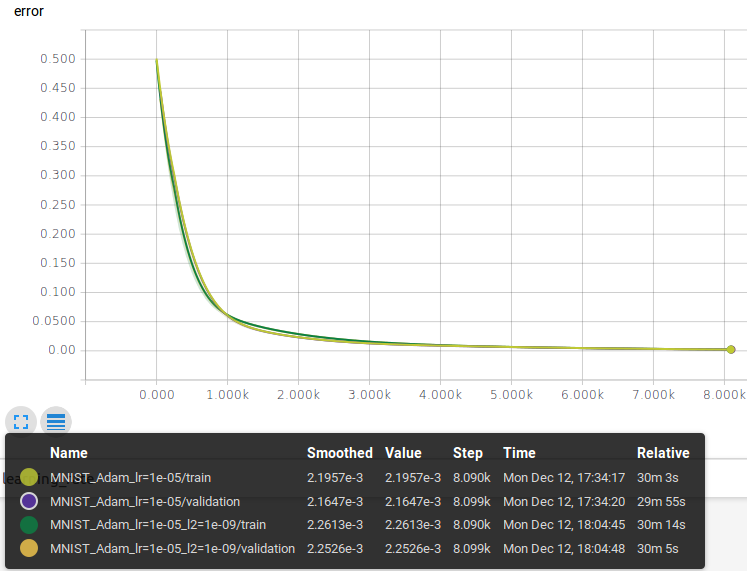
The graph shows 4 loss functions (reconstruction errors) that are the metrics we’re interested in to evaluate our models.

1. Training reconstruction error of the model without L2 penalty
2. Validation reconstruction error of the model without L2 penalty (with L2 disabled)
3. Training reconstruction error of the model with L2 penalty
4. Validation reconstruction error of the model with L2 penalty (with L2 disabled)

The functions have a similar trend, there’s only a small difference among them that’s due by the L2 regularization applied during the training phase.

DTB logs the reconstruction error achieved on the validation and test sets in validation_results.txt and test_results.txt files respectively.

The average reconstruction errors on the validation set at the end of the training process are:

• No regularization: 0.00216
• L2 regularization: 0.00225

The reconstruction error value on the test set is:

• No regularization: 0.00215
• L2 regularization: 0.00223

There’s a very small difference between the results achieved with and without L2: this can be a clue that the model has a capacity higher than the one required to solve the problem and the L2 regularization is pretty useless in this case.

It’s then possible to reduce the number of parameters and/or add a sparsity constraint to the loss, but this is left to the reader.

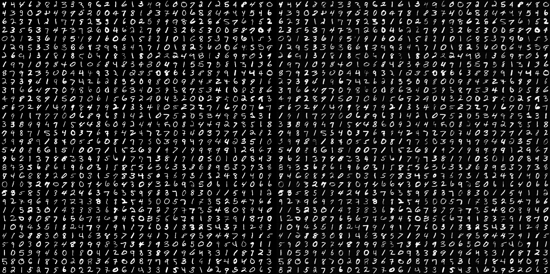
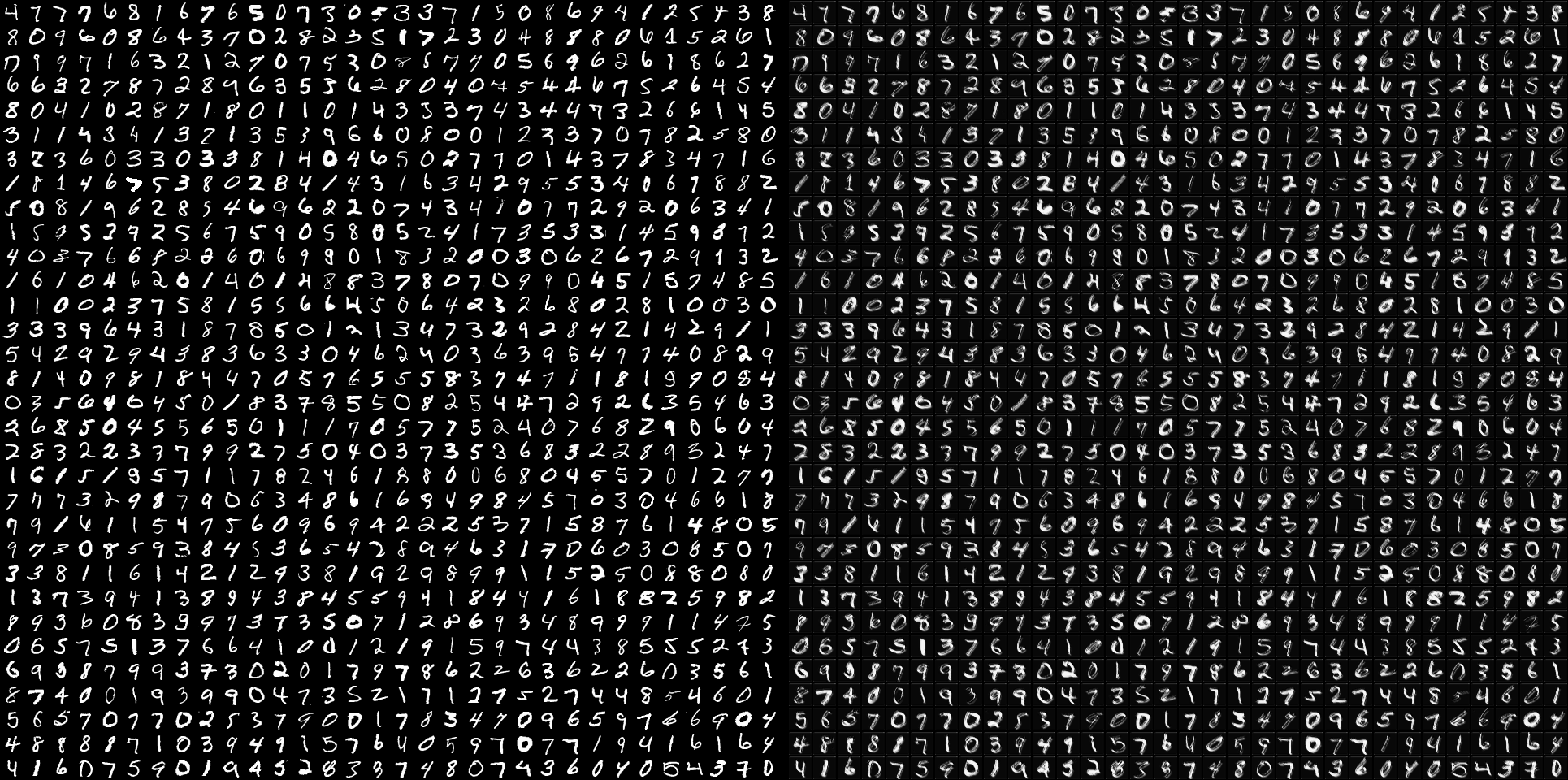
It’s possible to compare some input image and its reconstructed version for both models: DTB builds these visualizations for us.

Another visual feedback that helps to spot the differences between the two models is to see the learned filters together with their application to an input image before and after the activation function.

See what regions are active (different from 0) after the application of an activation function gives us the possibility to understand what neurons are excited from certain patterns in the input image.

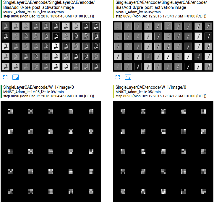
In the image we can see that the learned filters are different, but their combination is almost the same. A thing to note is that both models learned to reproduce the numbers (almost) correctly and the black background: this is because of the activation function added to the decoding layer. Previous tests with no activation applied showed how the CAE can learn to reproduce the numbers but not the background: it was gray instead of black. When the activation function is present, instead, it constrain the network to produce values that live in the same space of the input ones.

DTB gives us another feedback that’s helpful to deeply understand the pros and the cons of these implementations. The visualization of a single image, before and after the application function in the decoding layer.

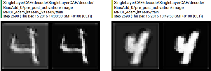
If we look carefully we can see that both models produce artifacts on the borders of the reconstructed images: this is due to the initial padding operation that forces the network to learn a padded, thus not real, representation of the input.

CIFAR 10

As we just did for the MNSIT dataset, let’s analyze in the same way the results obtained on the Cifar10 dataset.

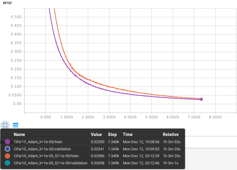
The graph shows the same 4 loss functions (reconstruction errors). With respect to the MNIST case, these losses are higher: they start from a high value and end at a higher value.

As in the MNIST case, the L2 penalty term affects the loss value making it higher.

The average reconstruction errors on the validation set at the end of the training process are:

• No regularization: 0.02541
• L2 regularization: 0.03058

In this case, the difference between the 2 model is somehow evident, the difference is about 1%.

The Cifar10 test set is the validation set, therefore there’s no need to rewrite the results.

We can visualize the comparison between the original and the reconstructed images as did before:

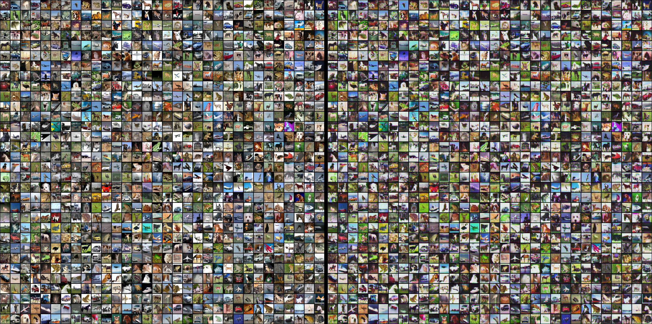
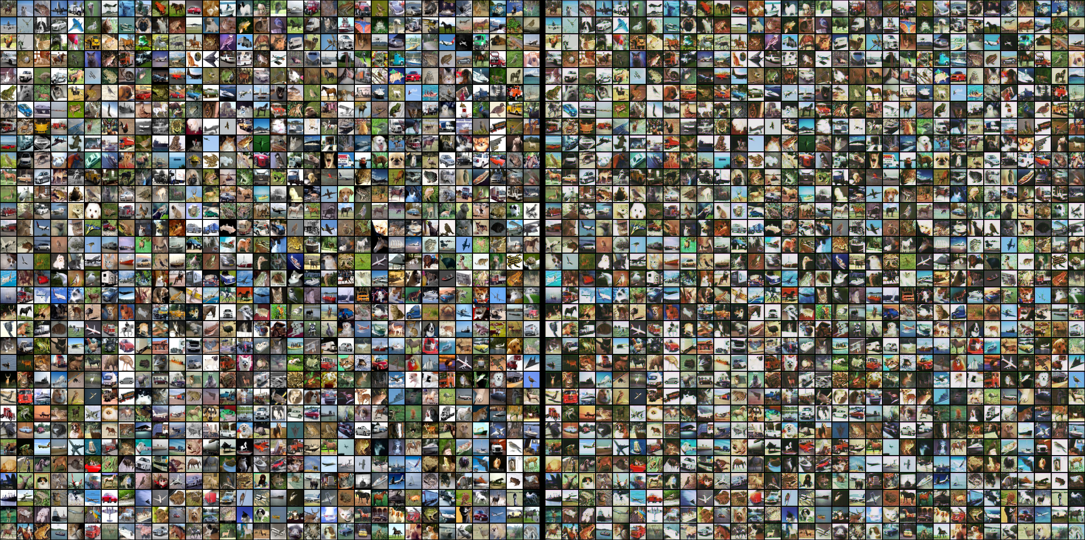
It’s possible to visualize the encoding filters learned and the activation maps produced:

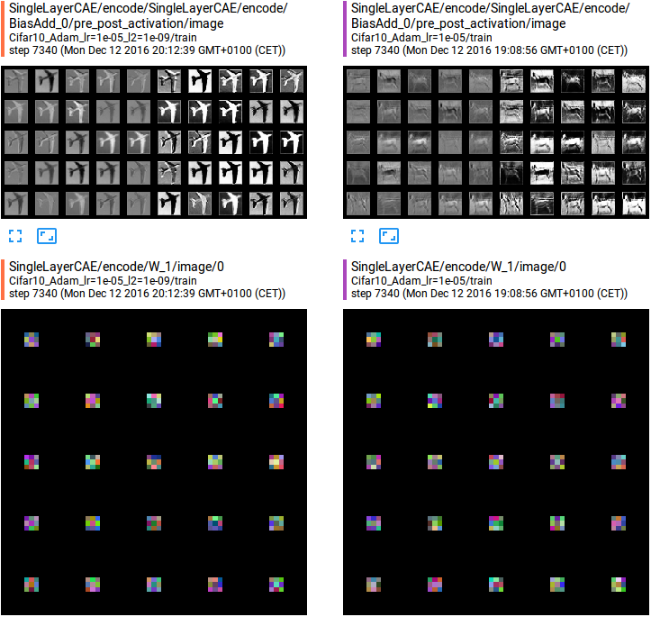
This case is more interesting of the MNIST one: looking at the activation maps produced when the input is an airplane, we can see that the network learned to somehow segment the airplane for the background or to do the contrary (being inactive when there’s an airplane but active when there’s light-blue background).

Even in this case, the learned filters among the two models are different, but the reconstruction is almost perfect in both cases as we can see from the images above.

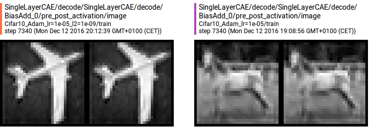
In this case, the artifacts introduced by the padding operation are less marked but still presents.

Conclusions

Tensorflow together with DTB can be used to easily build, train and visualize Convolutional Autoencoders. DTB allows experiencing with different models and training procedures that can be compared on the same graphs.

The created CAEs can be used to train a classifier, removing the decoding layer and attaching a layer of neurons, or to experience what happen when a CAE trained on a restricted number of classes is fed with a completely different input.

There are lots of possibilities to explore. If you have some ideas on how to use CAEs write them in the comment section!