Every Machine Learning (ML) product should reach its final stage: the deployment to production.
We all know that there is a lot of hype around the ML-based solutions (or with even more hype, the “AI-powered” solutions) and that everyone claims to have some fancy model in production. More than often, this is false1 and the development of the ML-based solution stops at the Jupiter Notebook where the scientists/researchers did their job.
Some lucky model, however, reaches the final stage - or because the management had a great plan (see video below), or because the model performed well and it passed all the QA steps.
Unfortunately, there isn’t a plethora of examples containing information on how to deploy a model to production and how to design the model environment for the production: all we can find is a bunch of articles on Medium that stops at the measurement of some metric on the validation set (some good person, at least, measures the performance on the test set).
In this article, I’m going to cover these points using TensorFlow 2 as the framework of choice and Go as the target language for the deployment - and training!

Note: the topic of deployment to production is broad and way more complex than what it’s presented in this article - in this article we can find the general guidelines for the design of the model, how to properly export and use a SavedModel, and how to deploy a model using Go - that’s fine for a small project, but it’s not representative of the real complexity of the whole MLOps pipeline (that not required, in any case, for the great majority of the ML projects - most of them, especially the project targeted for dedicated devices, can follow a simpler pipeline similar to the one presented in the article).
Human Activity Recognition
Let’s start with the most important advice: do not use Machine Learning if the problem you’re trying to solve can be solved with a decent accuracy with some good heuristic - or even worse, if the problem is solvable with a deterministic algorithm (it’s crazy, but we have to stress this since everyone is now throwing machine learning to every problem, even when it’s completely useless).
In our case, the problem we want to solve is human activity recognition from sensor data. We want to use data coming from an accelerometer to predict the activity the user is currently performing.
We want to first train the model on some labeled data and afterward use the deployed model to do incremental learning. With incremental learning we intend the continuous update of the model parameters (on the deployed model!), using new (labeled) data.
We suppose the user is wearing a generic “device” equipped with an accelerometer. This device is also our target deployment platform. We also suppose that the target device is able to run a Go program since we decided to use Go as target language.
The accelerometer gives us the acceleration values along the 3-axis, and the device accompany the acceleration data with the timestamp. Formally we have the endless acquisition \(A = (a_1, a_2, \cdots,)\) where \(a_i = (x_i, y_i, z_i, t_i)\) is a tuple with acceleration \((x_i, y_i, z_i) [\frac{m}{s^2}]\) at instant \(t_i\).
Luckily, there is a public domain dataset containing this kind of data we can use for running this simulation. The WISDM dataset introduced in the paper Activity Recognition using Cell Phone Accelerometers is our choice.
The (raw) dataset contains the following features:
user: An unique identifier of the user doing the activity.activity: The label for the current row. We have six different categories:walking,jogging,upstairs,downstairs,sitting, andstanding.timestamp: the time step \(t_i\) in which the accelerometer acquired the data.(x, y, z): the acceleration values along the 3 axes (at the time step \(t_i\)).
The process of data acquisition has been documented and we have a nice YouTube video showing it:
Note: in the real scenario, starting from a public domain dataset it might be the correct choice if the domain of application is very very similar and the process of transfer learning / fine-tuning is thus applicable. Otherwise, if you have some raw data without labels and you don’t have any ready-to-use dataset, perhaps it is worth to annotate the raw data - it can save you a lot of time in the long run.
Looking at the dataset structure, we can see we have a CSV file (WISDM_ar_v1.1_raw.txt) that contains all the features previously described:
| ID | Activity | Timestamp | X | Y | Z |
|---|---|---|---|---|---|
| 33 | Jogging | 49105962326000 | -0.6946377 | 12.680544 | 0.50395286; |
| 33 | Jogging | 49106062271000 | 5.012288 | 11.264028 | 0.95342433; |
| 33 | Jogging | 49106112167000 | 4.903325 | 10.882658 | -0.08172209; |
| … | … | … | … | … | … |
As we can see, the final value contains a ; that should be removed. However, to make the processing more fun, instead of doing it in Python, we’ll do it using Go - as well as the training phase (!).
Note: The article contains the full training process (without metric measurement, model selection, and so on) in Go, just to show how it’s possible to export into a SavedModel very complex functions and how to design the
tf.Modulefor this task. However, the correct training procedure (with dataset split, validation, metric measurement, model selection, and cross-validation) it’s the recommended path to follow and to do in Python.
Model definition
There are tons of architecture that can solve this task pretty well: we have RNNs and bidirectional-RNNs that are the standard de-facto for time series classification. In this article we don’t focus that much on the architecture since it’s not the main topic - we’ll use an RNN just to have a small model and to train it easily. Perhaps a bidirectional-RNN would be better since the architecture takes into account the future data (w.r.t. the current timestep \(t_i\)).
We define this dummy model using the Keras Sequential API: the idea is to do not reset the state of the model until we change the activity - in this way we can train the RNN making it see the complete sequence of sensor data per activity and per user.
In order to be production-oriented - that in this context means to be ready to export the model itself - we define it inside a tf.Module. Placing the model inside a tf.Module is not required if we are interested in exporting only the model, because the Keras API supports it out of the box. However, since we are interested in exporting the training loop we want to put the model, the training step, and all the required dependencies for the training (and inference) inside a tf.Module.
import sys

import tensorflow as tf
import tensorflow.keras as k


class ActivityTracker(tf.Module):
    def __init__(self):
        super().__init__()

        self.num_classes = 6  # activities in the training set
        self.num_features = 3  # sensor (x,y,z)

        # NOTE: we need a fixed batch size because the model has a state
        self.batch_size = 32
        self._model = k.Sequential(
            [
                k.layers.Input(
                    shape=(1, self.num_features),
                    batch_size=self.batch_size,
                ),
                # Note the stateful=True
                # we'll reset the states and the end of the per-user activity sensor data
                k.layers.LSTM(64, stateful=True),
                k.layers.Dense(self.num_classes),
            ]
        )
The model, I repeat, is dummy - but I won’t be surprised if that simple model is able to solve the problem as well.
In the __init__ method, we also want to add all the stateful objects, because as explained in Analyzing tf.function to discover AutoGraph strengths and subtleties - part 1: Handling states breaking the function scope when we convert the eager code to its graph representation, every Python tf.Variable definition defines a new graph node, but we don’t want to create a new node every time we invoke a function
Note: We must design our production-oriented code in this way from the beginning, always thinking about the graph representation, otherwise we’ll find ourselves rewriting everything from scratch in a final rush when it’s time to deploy.
Moreover, we also want to add to the tf.Module all the objects we want to serialize together with the model. Thus, since we are interested in serializing the whole training loop, we add:
- The optimizer (
self._optimizer) - The loss function (
self._loss) - The training steps counter (
self._global_step) - A variable containing the last tracked activity - we use this variable to reset the model state when it’s the right time (
self._last_tracked_activity) - A handy StaticHashTable that maps the scalars \([0, 6[\) to the corresponding textual representation of the labels.
        self.mapping = tf.lookup.StaticHashTable(
            tf.lookup.KeyValueTensorInitializer(
                keys=tf.range(self.num_classes, dtype=tf.int32),
                values=[
                    "Walking",
                    "Jogging",
                    "Upstairs",
                    "Downstairs",
                    "Sitting",
                    "Standing",
                ],
            ),
            "Unknown",
        )

        self._global_step = tf.Variable(0, dtype=tf.int32, trainable=False)
        self._optimizer = k.optimizers.SGD(learning_rate=1e-4)
        # Sparse, so we can feed the scalar and get the one hot representation
        # From logits so we can feed the unscaled (linear activation fn)
        # directly to the loss
        self._loss = k.losses.SparseCategoricalCrossentropy(from_logits=True)

        self._last_tracked_activity = tf.Variable(-1, dtype=tf.int32, trainable=False)
All the stateful objects and utility attributes have been defined, we are now ready to define two graphs:
- The training step: this graph is just a single training step.
- The inference: this graph takes the input and returns a single prediction (the label resulting from the prediction over the whole input timesteps).
Before defining the graph, first a small digression about tf.function
All in graph
As explained in part 1, part 2, and part 3 of the article Analyzing tf.function to discover AutoGraph strengths and subtleties and summarized in the talk Dissecting tf.function to discover AutoGraph strengths and subtleties we have to design our functions thinking about the graph representation, otherwise we will have a hard time to convert our code to its graph-convertible counterpart.
The second most important thing to remember (the first one is how to deal with functions that create a state) is that we have to use as many TensorFlow primitive operations as we can, instead of using the Python one. In fact, the Python code is executed during the first invocation of the function (with a certain input and type, as explained in the previously linked articles) and the function execution is traced while the tf.Graph get’s created.
Thus, when we define our train step graph and inference graph, we’ll use all the tf.* operation instead of the Python operations (e.g. tf.range instead of range, tf.assert instead of assert, …).
Train step graph & SignagureDef
We want to design our learn function as a training step over a batch of data. We have to be sure that all the data in the batch is data coming from the same activity (thus they all have the same label), and we want to take care of the state of the training by changing the value of self._last_tracked_activity if the current batch is labeled as a new activity (respect to the previously seen batch), and resetting the RNN state.
The training step is pretty common so we won’t focus on it (the code is pretty clear), but the interesting part of the snippet below is the tf.function decoration with the input_signature specification, together with the return value (the loss) that’s a dict.
Defining the input_signature of a tf.function-decorated function is mandatory to correctly export the function as a graph in the SavedModel.
A SavedModel contains a complete TensorFlow program, including weights and computation. It does not require the original model building code to run, which makes it useful for sharing or deploying2
Without this specification, the SavedModel will contain only a section called “functions” that are not usable outside of a Python environment.
The input_signature parameter must define the input shape and type we require for the graph. Since this is a training step, we need a batch of data with shape \((\text{None}, 1, 3)\) since we want to feed this data to an RNN one observation at a time, where every observation is composed by the \((x,y,z)\) values of the sensor data.
The return value of this function is the loss value, wrapped in a dictionary. Wrapping it in a dictionary is not mandatory, but it’s recommended.
Defining the input_signature parameter of tf.function together with the usage of a dictionary to create a pair (key, value) for the return value, is the process of definition of the so-called SignatureDef.
A SignatureDef defines the signature of a computation supported in a TensorFlow graph. SignatureDefs aim to provide generic support to identify inputs and outputs of a function and can be specified when building a SavedModel.
More information about the SignatureDef are available in the TFX tutorial: SignatureDefs in SavedModel for TensorFlow Serving
    @tf.function(
        input_signature=[
            tf.TensorSpec(shape=(None, 1, 3), dtype=tf.float32),
            tf.TensorSpec(shape=(None,), dtype=tf.int32),
        ]
    )
    def learn(self, sensor_data, labels):
        # All the sensor data should be about the same activity
        tf.assert_equal(labels, tf.zeros_like(labels) + labels[0])

        # If the activity changes, we must reset the RNN state since the last update
        # and the current update are not related.

        if tf.not_equal(self._last_tracked_activity, labels[0]):
            tf.print(
                "Resetting states. Was: ",
                self._last_tracked_activity,
                " is ",
                labels[0],
            )
            self._last_tracked_activity.assign(labels[0])
            self._model.reset_states()

        self._global_step.assign_add(1)
        with tf.GradientTape() as tape:
            loss = self._loss(labels, self._model(sensor_data))
            tf.print(self._global_step, ": loss: ", loss)

        gradient = tape.gradient(loss, self._model.trainable_variables)
        self._optimizer.apply_gradients(zip(gradient, self._model.trainable_variables))
        return {"loss": loss}
The definition of the training loop in Python, with the creation of the tf.data.Dataset object, the proper validation, and model selection of the best model is left as an exercise to the reader :)
We will cover the training part directly in Go - but here’s a spoiler: it won’t be persistent on the disk, because the support Go side (and tfgo side) is not completed yet - that’s why I recommend doing the complete training in Python (want to contribute? continue reading the article, find the tfgo repository link and let’s talk there!).
The inference graph
The inference graph SignatureDef definition follows the very same rules used for the train step graph - the only difference is in the input/output parameters of course. In this case, we want to return the majority class predicted for the set of activities in the batch.
In this function, we also use the mapping created in the __init__ to print the textual representation of the prediction.
    @tf.function(input_signature=[tf.TensorSpec(shape=(None, 1, 3), dtype=tf.float32)])
    def predict(self, sensor_data):
        predictions = self._model(sensor_data)
        predicted = tf.cast(tf.argmax(predictions, axis=-1), tf.int32)
        tf.print(self.mapping.lookup(predicted))
        return {"predictions": predicted}
Note: printing in the graph is not recommended (although it’s very useful to understand what’s going on) because it’s a side effect that the target platform/language should handle and perhaps is not always easy to do it.
Export everything as a SavedModel
After having defined everything inside a tf.Module and having correctly decorated the functions we want to export as graphs, all we need to do is to use the tf.saved_model.save function.
Since we are exporting a tf.Module we have to remember that the default behavior is to do not export the serving signature defs (that are handy entry points inside the SavedModel that tools like saved_model_cli and to Go bindings (and all the others) can use to load the correct graph from the SavedModel), and thus we have to explicit the signatures by ourselves.
Important: the process of graph creation is executed only after the function execution is traced, we have to run the functions with some dummy input (but with the correct shape and dtype).
def main() -> int:
    at = ActivityTracker()

    # Executing an invocation of every graph we want to export is mandatory
    at.learn(
        tf.zeros((at.batch_size, 1, 3), dtype=tf.float32),
        tf.zeros((at.batch_size), dtype=tf.int32),
    )
    at.predict(tf.zeros((at.batch_size, 1, 3), dtype=tf.float32))

    tf.saved_model.save(
        at,
        "at",
        signatures={
            "learn": at.learn,
            "predict": at.predict,
        },
    )

    return 0


if __name__ == "__main__":
    sys.exit(main())
Saving the file as export.py and executing it with python export.py we end up with the at folder inside our current working directory that contains our SavedModel.
SavedModel inspection
Before jumping in the Go code and defining the training loop and using the graphs we just defined, we have to analyze the SavedModel created to see:
- The exported tag (that’s by default one, the
"serve"tag) - The exported graphs
- The input/output tensor to use to feed the graph / get the results.
The tool to use is saved_model_cli that comes with the Python installation of TensorFlow.
saved_model_cli show --all --dir at
The CLI tool gives us this information:
signature_def['learn']:
  The given SavedModel SignatureDef contains the following input(s):
    inputs['labels'] tensor_info:
        dtype: DT_INT32
        shape: (-1)
        name: learn_labels:0
    inputs['sensor_data'] tensor_info:
        dtype: DT_FLOAT
        shape: (-1, 1, 3)
        name: learn_sensor_data:0
  The given SavedModel SignatureDef contains the following output(s):
    outputs['loss'] tensor_info:
        dtype: DT_FLOAT
        shape: ()
        name: StatefulPartitionedCall_1:0
  Method name is: tensorflow/serving/predict

signature_def['predict']:
  The given SavedModel SignatureDef contains the following input(s):
    inputs['sensor_data'] tensor_info:
        dtype: DT_FLOAT
        shape: (-1, 1, 3)
        name: predict_sensor_data:0
  The given SavedModel SignatureDef contains the following output(s):
    outputs['predictions'] tensor_info:
        dtype: DT_INT32
        shape: (-1, 1)
        name: StatefulPartitionedCall_2:0
  Method name is: tensorflow/serving/predict
We have our 2 SignatureDef defined previously, with the input name taken from the input parameters name, and the output is taken from the keys in the return dict we used (loss and predictions).
Note: we are interested in the name section of every input/output. This name is the name of the tf.Tensor that we have to use to feed the model (for the inputs) or for getting the result (for the output nodes).
The :0 (or in general :<suffix>) is a progressive number that indicates how many outputs the operation (a tf.Operation is a node that produces 0 or more tf.Tensor) produces.
The simulation of the real case scenario
In this article, we simulate the real scenario in which we suppose the user wears this device equipped with an accelerometer.
- The user device gathers the data during an activity.
- At the end of the activity, we perform an inference step and try to label the sensor data (
Observations) received. - We ask the user if the predicted label is the correct one. If it’s not, we ask the user to choose the correct label.
- With the data and the label, we perform a training step to adapt the model parameters to the user-generated data.
In this way, in the long run, the model will predict the correct label for the tracked activity, even if the user exhibits an unusual pattern in the observations (this might be the case of people with disabilities or athletes).
But first, we perform the training directly in Go :)
Note: as anticipated, the persistence of the trained model is not possible for now, thus it’s better to train the model in Python - in the article we’ll show, however, how it’s possible to train a model from Go (the persistence part needs your help!)
Training and Inference in Go with tfgo
The setup of the Go environment and the installation of the TensorFlow’s C library goes beyond the scope of this article and it won’t get covered.
I just leave a link to the project I maintain, tfgo, that allows not to install the official TensorFlow Go package (because it’s not go-gettable, see #39307, #41808, #35133) and it gives to you, as a dependency automatically installed by go get, a working version of the tensorflow package together with all the features exposed by the tfgo package.
Just a small note, the fork that is automatically installed when go-getting tfgo is just a fork of the TensorFlow repository (branch r2.3) that contains all the compiled protobuf files needed to make go-gettable the package.
From the SavedModel inspection, we know everything we need to use the graphs we defined.
We begin with the various import we’ll use throughout the main package, and we start with the definition of the Observation struct that maps a row of the dataset to a Go type, and the of the batchSize constant (that should be as such because the RNN is stateful).
package main

import (
	"encoding/csv"
	tg "github.com/galeone/tfgo"
	tf "github.com/tensorflow/tensorflow/tensorflow/go"
	"io"
	"log"
	"math/rand"
	"os"
	"strconv"
	"strings"
	"time"
)

type Observation struct {
	ID        int
	Activity  string
	Label     int32
	Timestamp time.Time
	X         float32
	Y         float32
	Z         float32
}

const batchSize int = 32
We can now start wrapping the model graphs using the *tfgo.Model functions. The predict function is pretty easy and it doesn’t require any explanation, just note that we extract with model.Op the operation names (followed by the suffix 0 in this case) from the graph, and we use these operations to get the Tensors to use for the model input/output.
// predict invokes the predict method of the model and returns the majority class
// predicted for the input batch.
//
// model: the *tg.Model to use
// sensorData: a tf.Tensor with shape (32, 1, 3)
func predict(model *tg.Model, sensorData *tf.Tensor) int32 {
	predictions := model.Exec([]tf.Output{
		model.Op("StatefulPartitionedCall_2", 0),
	}, map[tf.Output]*tf.Tensor{
		model.Op("predict_sensor_data", 0): sensorData,
	})[0].Value().([][]int32)

	var votes map[int32]int
	votes = make(map[int32]int)
	for i := 0; i < len(predictions); i++ {
		votes[predictions[i][0]]++
	}

	var maxVote int = -1
	var topLabel int32 = 0
	for label, vote := range votes {
		if vote > maxVote {
			maxVote = vote
			topLabel = label
		}
	}
	return topLabel
}
The predict function works on the raw *tf.Tensor, so we can define a utility function observationsToTensor and hide the raw *tf.Tensor with a new Predict function that works, instead, with a batch of observations.
func observationsToTensor(observations [batchSize]Observation) *tf.Tensor {

	var sensorData [batchSize][1][3]float32
	size := len(observations)
	if size < batchSize {
		log.Fatalf("Observations size %d < batch size %d", size, batchSize)
	}

	for i := 0; i < size; i++ {
		sensorData[i][0] = [3]float32{observations[i].X, observations[i].Y, observations[i].Z}
	}

	var err error
	var sensorTensor *tf.Tensor

	if sensorTensor, err = tf.NewTensor(sensorData); err != nil {
		log.Fatal(err)
	}

	return sensorTensor
}

func Predict(model *tg.Model, observations [batchSize]Observation) int32 {
	sensorData := observationsToTensor(observations)
	return predict(model, sensorData)
}
To Go code is really easy to read and understand, the only peculiarity is that we must always use the Go type that corresponds to the correct type expected by the graph, otherwise the *tg.Model.Exec call will panic. The panic is caused by the underlying TensorFlow C library that returns an error code and the model just forwards the error message to the caller.
The same reasoning must be applied in the opposite direction: the invocation of *tf.Tensor.Value() returns an interface{} type and we must access the underlying value doing the correct type assertion to avoid panics.
We can do the very same reasoning for the training graph. We have in our SavedModel a graph that’s a training step, and we can use it in the very same way we use the prediction graph.
// learn runs an optimization step on the model, using a batch of values
// coming from the same observed activity.
// NOTE: all the observations must have the same label in the same batch.
//
// model: the *tg.Model to use
// sensorData: a tf.Tensor with shape (32, 1, 3)
// labels: a tf.Tensor with shape (32)
func learn(model *tg.Model, sensorData *tf.Tensor, labels *tf.Tensor) float32 {
	loss := model.Exec([]tf.Output{
		model.Op("StatefulPartitionedCall_1", 0),
	}, map[tf.Output]*tf.Tensor{
		model.Op("learn_sensor_data", 0): sensorData,
		model.Op("learn_labels", 0):      labels,
	})[0]

	return loss.Value().(float32)
}

func Learn(model *tg.Model, observations [batchSize]Observation) float32 {
	var sensorData [batchSize][1][3]float32
	var labels [batchSize]int32

	for i := 0; i < batchSize; i++ {
		sensorData[i][0] = [3]float32{observations[i].X, observations[i].Y, observations[i].Z}
		labels[i] = observations[i].Label
	}

	var err error
	var sensorTensor *tf.Tensor
	var labelTensor *tf.Tensor

	if sensorTensor, err = tf.NewTensor(sensorData); err != nil {
		log.Fatal(err)
	}
	if labelTensor, err = tf.NewTensor(labels); err != nil {
		log.Fatal(err)
	}

	return learn(model, sensorTensor, labelTensor)

}
We now have all we need to define the training function we use to run one epoch of training.
Training loop definition in Go
Our goal is to parse every row of the training set (CSV), skip errors that ARE present in the dataset structure, and use the Observation to train the model.
We can start, thus, defining the NewObservation constructor that instantiates an *Observation from a []string and a map that contains the mapping ID -> textual label.
func NewObservation(record []string, mapping map[string]int32) (*Observation, error) {
	var err error
	var id int
	if id, err = strconv.Atoi(record[0]); err != nil {
		return nil, err
	}

	activity := strings.ToLower(record[1])

	var sec int
	if sec, err = strconv.Atoi(record[2]); err != nil {
		return nil, err
	}

	var x, y, z float64

	if x, err = strconv.ParseFloat(record[3], 32); err != nil {
		return nil, err
	}

	if y, err = strconv.ParseFloat(record[4], 32); err != nil {
		return nil, err
	}

	if z, err = strconv.ParseFloat(strings.TrimRight(record[5], ";"), 32); err != nil {
		return nil, err
	}

	return &Observation{
		ID:        id,
		Activity:  activity,
		Label:     mapping[activity],
		Timestamp: time.Unix(int64(sec), 0),
		X:         float32(x),
		Y:         float32(y),
		Z:         float32(z),
	}, nil
}
The training loop can now be easily defined: we build the batch, run the training step, and assure that every value in the batch has the same label (and comes from the same user).
func train(model *tg.Model, datasetPath string, mapping map[string]int32) {
	var err error
	var filePtr *os.File

	if filePtr, err = os.Open(datasetPath); err != nil {
		log.Fatal(err)
	}

	defer func() {
		if err := filePtr.Close(); err != nil {
			log.Fatalf("close: %s", err)
		}
	}()

	reader := csv.NewReader(filePtr)

	var record []string
	var read int

	var user int
	var label int32

	var observations [32]Observation

	for {
		record, err = reader.Read()
		if err == io.EOF {
			break
		}

		if err != nil {
			log.Fatal(err)
		}

		var o *Observation
		if o, err = NewObservation(record, mapping); err != nil {
			log.Printf("Skipping observation %v", record)
			continue
		}
		read++
		// Set the user for the current set of observations
		// The user and the label must be the same for all the training batch
		if read == 1 {
			user = o.ID
			label = o.Label
		}

		if user != o.ID || label != o.Label {
			if user != o.ID {
				log.Printf("Changing user %d -> %d\n", user, o.ID)
			}
			if label != o.Label {
				log.Printf("Changing label %d -> %d\n", label, o.Label)
			}
			read = 1
			user = o.ID
			label = o.Label
		}

		observations[read-1] = *o

		if read == batchSize {
			Learn(model, observations)
			read = 0
		}
	}
}
Here we go: we are ready to invoke our train function and use Go to train the model.
func main() {
	mapping := map[string]int32{
		"walking":    0,
		"jogging":    1,
		"upstairs":   2,
		"downstairs": 3,
		"sitting":    4,
		"standing":   5,
	}

	var model tg.Model = *tg.LoadModel("at", []string{"serve"}, nil)

	train(&model, "WISDM_ar_v1.1/WISDM_ar_v1.1_raw.txt", mapping)
Running the code written so far, we can see the training loop working, the internal states changing, and everything going as expected :)
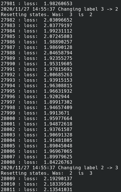
I highlight again that this is just an example to show how to design a training loop with TensorFlow and Go - it lacks all the minimal features we need for correct training.
Simulating the user interaction
The user interaction is just simulated and also the sensor data is randomly generated, however, in the following lines of code, we can see how easy it by using Go to receive the observations from a chan and do a prediction over this received data.
The prediction is sent back over a channel to be displayed to the user, and if the user accepts (or changes the label) the new training data is sent to a go-routine that invokes the Learn function with this new set of observations, to iteratively refine the model and customizing it on the user behavior.
	// With a trained model, we are ready to receive other observations
	// and use them to train it during its lifetime.

	observations := make(chan Observation, batchSize)
	prediction := make(chan int32, 1)

	go func() {
		var obs [batchSize]Observation
		for i := 0; i < batchSize; i++ {
			obs[i] = <-observations
		}

		prediction <- Predict(&model, obs)
		// requeue all the observations in the same channel
		// in order to let other routines to use the same
		// observations (for training with the predicted/adjusted label)
		for i := 0; i < batchSize; i++ {
			observations <- obs[i]
		}

	}()

	done := make(chan bool, 1)
	go func() {
		// This is an example of a real case
		// where the sensor is gathering some data
		// and the user labels it (perhaps after our model suggestion that
		// can be used as a hint for the user to set the label :) ).

		// This function generates the data of the activity
		// and sends a batch of this data in the observation channel.

		// On the other side of the channel we have the model waiting
		// for this data, that sends back a suggested label and waits for a
		// user confirmation.

		// Generate sensor data

		var min, max float32 = 1, 10
		rand.Seed(time.Now().UnixNano())

		for i := 0; i < batchSize; i++ {
			x := min + rand.Float32()*(max-min)
			y := min + rand.Float32()*(max-min)
			z := min + rand.Float32()*(max-min)

			observations <- Observation{
				Timestamp: time.Now(),
				X:         x,
				Y:         y,
				Z:         z,
			}
		}

		predictedLabel := <-prediction
		log.Printf("predicted label: %d", predictedLabel)

		// In the real case, the predicted label is asked for
		// confirmation to the user and if the user accepts the suggestion
		// the model is trained with the current set of the observations
		// and the confirmed label (or the new label given by the user)

		var obs [batchSize]Observation
		for i := 0; i < batchSize; i++ {
			obs[i] = <-observations
			obs[i].Label = predictedLabel
		}

		Learn(&model, obs)
		// Here we terminarte the application, but in the real scenario
		// this is an endless loop with frequent checkpoints
		// and model versioning.
		done <- true
	}()

	<-done

}
The code contains some (I hope helpful) comments to understand how to organize the message exchange and the whole application in the real scenario.
The complete go code is available here: device.go.
Conclusion
Designing code that can be exported as a SavedModel requires thinking about the graph representation - every production-oriented ML code should be designed with the graph in mind.
The SavedModel format contains a TensorFlow program: it’s not limited to the model inference, we can save everything that’s graph-convertible inside it. We have to take care of the SignatureDef and the peculiarities of tf.Module but this comes with the great advantage of being able to deploy this tf.Module everywhere.
Using tfgo it’s possible to have a working version of the official tensorflow go package, with a single go get, together with all the additional features of tfgo.
It’s possible to train a model in Go (although not recommended until we can save the status of a SavedModel) and in general, it’s really easy to use any graph defined inside a tf.Module if it has been correctly designed and exported.
The Go Philosophy of “Don’t communicate by sharing memory; share memory by communicating” fits well with the interactions that an ML model has with its deploy environment, especially if we are interested in incremental learning.
Disclaimer: The actual Python code executed in the article is not an RNN but I replaced the RNN with a Dense layer. Not for my choice but because TensorFlow has an open bug with the deployment of RNNs that should be addressed ASAP in my opinion (after all, this bug is preventing the deployment of stateful RNNs :S): #44428 - unfortunately the bug is still open and not addressed after 29 days (at the time of writing).